Information decomposition

Where is the information in data?

University of Pennsylvania

How to decompose the information contained in data about a relationship between multiple variables, by using the Distributed Information Bottleneck as a novel form of interpretable machine learning.

Papers | Code | Method overview

Papers

	Machine-learning optimized measurements of chaotic dynamical systems via the information bottleneck Physical Review Letters (Accepted) [arxiv link]
	Information decomposition in complex systems via machine learning PNAS 2024 [PNAS (open access)] \|\| [arxiv link]
	Interpretability with full complexity by constraining feature information ICLR 2023 [Conference proceedings link (OpenReview)] \|\| [arxiv link]
	Characterizing information loss in a chaotic double pendulum with the Information Bottleneck NeurIPS 2022 workshop "Machine learning and the physical sciences", selected for oral presentation [arxiv link]
	The Distributed Information Bottleneck reveals the explanatory structure of complex systems [arxiv link]

Code

Code is available on github!

Method overview

TL;DR Introduce a penalty on information used about each component of the input. Now you can see where the important information is.

We are interested in the relationship between two random variables \(X\) and \(Y\), which we'll call the input and output. We assume \(X\) is composite: there are components \(\{X_i\}\) that are measured together, that can have arbitrarily complex interaction effects with respect to the outcome of \(Y\).

Illustration of components of X interacting as a network culminating in Y — The components of \(X\) can have complex interaction effects with respect to the outcome of \(Y\).

This setting is ubiquitous. Some examples we have investigated:

\(\{X_i\}\)	\(Y\)
Density variations describing local structure in a glassy material Horizontal and vertical coordinates of position in an image Angles, velocities for arms of a double pendulum Stats for a hospital patient such as age, temperature, and P/F ratio Measurements of a sample of red wine	Whether that part of the material is about to rearrange Color at that point in the image Future state of double pendulum Outcome of treatment Rating of the wine

Given data of \(X\) and \(Y\), the typical route a machine learning practitioner takes is to fit a deep neural network to predict \(Y\) given \(X\). The resulting model is incomprehensible, however, granting predictive power without insight.

Schematic of components of X feeding into a neural network to predict Y — Typical machine learning setup: just feed it all in.

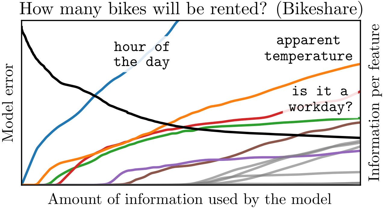
What we propose is to add a penalty during training: the model has to pay for every bit of information used about any of the \(\{X_i\}\). This has two powerful consequences: 1) The most predictive information is found, revealing the essential parts of the relationship, and 2) We gain a means to control the amount of information used by the machine learning model, yielding a spectrum of approximate relationships that serves as a soft on-ramp to understanding the relationship between \(X\) and \(Y\).

Schematically it looks like the following:

Schematic of components of X encoded by their own neural networks, then combined to predict Y — Distributing information bottlenecks to the features: one encoder and an information penalty each, then integrate all the information for prediction.

Each component \(X_i\) is compressed independently of the rest by its own encoder. The amount of information in the encodings is penalized in the same way as a Variational Autoencoder (VAE). All encodings \(\{U_i\}\) are then aggregated and used to predict \(Y\).

We track the flow of information from the components by varying the information alloted to the machine learning model. Shown below is one example: a Boolean circuit with 10 binary inputs routing through various logic gates to produce the output \(Y\).

Boolean circuit with 10 inputs routing through multiple logic gates to produce output Y. Plot showing the information allocation to the input components found by the distributed information bottleneck method. — Reverse engineering a Boolean circuit by tracking information about the inputs.

By training with the Distributed IB on input-output data we find the most informative input gate is number 3 (green), followed by number 10 (cyan), and so on. As more information is used by the machine learning model, its predictive power grows until it uses information from all 10 input gates.